Snow Fall Scenes Saver serial key or number

SC losses

Figure 1b shows the boxplot of the dry-season SC extent retrieved from Landsat imagery over the 22 zones indicated in Fig. 1a, over two periods: 1986–2005 (red) and 2006–2015 (blue). As shown in Fig. 1b, the dry-season SC extent in the northern Atacama Desert (18°–23°S) tends to be significantly lower than in extratropical zones (23–34°S). The relatively low SC values from latitude 18°S to latitude 23°S are consistent with the fact that in the Tropics, Andean snow is constrained to high elevations (>5000 m)^8,9. Due to higher precipitation and lower temperatures (compared to the northern Atacama Desert)³⁹, the Andean dry-season SC peaks at extratropical latitudes (23°–34°S), then slightly decreasing again at mid-latitudes (34°–40°S).

Figure 1b also allows assessing the significant losses in the SC extent in recent decades across the entire study area. Comparing the boxes computed over the periods 1986–2005 (red) and 2006–2015 (blue), it can be observed that the distribution of the SC retrievals shifted toward lower values in almost all zones. This shifting has increased the likelihood of low SC values during the dry-season. According to Fig. 1b, in each of the 22 zones within our study area (especially in the northern Atacama Desert), low dry-season SC values are significantly more likely nowadays than over the base period 1986–2005.

Figure 1b shows that the dry-season SC extent declined in recent decades in our study area: about 39% at tropical latitudes (18°–23°S), and more than 19% at extratropical and mid-latitudes (23°–40°S). Note that these changes are likely influenced by the drought that affected the region since 2010⁴⁰.

Correlation with climate indices

We tested the correlations between the dry-season SC extent (in the 3 macrozones considered in this study) and 3 climate indices: the SST anomaly in the Niño 1 + 2 region (0–10°S, 90°W–80°W)⁴¹, the Southern Oscillation Index (SOI)⁴², and the SAM index⁴³. Weekly SST anomalies in the Niño regions were provided by NOAA’s Climate Prediction Center (CPC): https://www.cpc.ncep.noaa.gov/data/indices/wksst8110.for; monthly SOI values were provided by NOAA’s National Center for Environmental Information: https://www.ncdc.noaa.gov/teleconnections/enso/indicators/soi/data.csv; and monthly SAM data were provided by NOAA’s Earth System Research Laboratory: https://www.esrl.noaa.gov/psd/data/20thC_Rean/timeseries/monthly/SAM/. Figure 2 shows the time series of the dry-season SC extent (averaged over each of the 3 macrozones considered in this study) and the time series of the SST anomaly in the Niño 1 + 2 region (first row), the SOI values (second row), and the SAM index (third row). The correlation coefficients (R) are shown in the upper right corner of each plot.

Figure 2 confirms a relatively good correlation between the dry-season SC extent at extratropical latitudes and the SST anomaly in the Niño 1 + 2 region (see Fig. 2a). This is not surprising since the Niño 1 + 2 region corresponds to the equatorial Pacific coast of South America⁴¹. The correlation between ENSO/El Niño indices and the Andean SC extent at tropical/extratropical latitudes has been widely confirmed^8,20,22. The strong correlation between the Andean snow persistence and SST anomalies in the Niño 1 + 2 region has been also previously highlighted²³. As shown in Fig. 2d, the correlation between the dry-season SC extent and the SST anomaly in the Niño 1 + 2 region is lower at higher latitudes (34°–40°S).

The correlation between the SOI values and the dry-season SC extent is not particularly strong (see Fig. 2b,e). The SOI value depends on the observed sea level pressure differences between Darwin (Australia) and Tahiti⁴². The SOI corresponds to the fluctuations in air pressure between the eastern and western tropical Pacific during the ENSO phases⁴². A stronger correlation between the SOI values and the snow persistence at extra-tropical latitudes has been previously reported²³ but that involved a different time scale.

Figure 2 also confirms a relatively high correlation between the SAM index and the dry-season SC extent at mid-latitudes (see Fig. 2f). The SAM index is defined as the difference of zonal mean sea level pressure between 40°S and 65°S⁴³; a positive index (lower polar pressure) is associated with weaker zonal winds while a negative value is associated with stronger zonal winds⁴³. The SAM influence on the SC extent at latitudes higher than 34°S was expected since the westerlies modulate the precipitation regime over the southeast Pacific²⁸. The good correlation between the SC at mid-latitudes and the SAM index has also been reported in prior efforts^8,23.

SC trends

Figure 3 (first row) shows the dry-season SC anomalies computed for our 3 macrozones: tropical latitudes (18°–23°S), extratropical latitudes (23°–34°S), and mid-latitudes (34°–40°S). As shown in Fig. 3 (first row), the dry-season SC extent exhibits decreasing trends in each of our 3 macrozones: about −16% per decade at tropical latitudes (18°–23°S), approximately −10% per decade at extratropical latitudes (23°–34°S), and about −15% per decade at mid-latitudes (34°–40°S). The significance of these trends was tested by using the Mann-Kendall (M-K) test⁴⁴. Despite the interannual variability, the trends are statistically significant (see Table 1), especially at tropical latitudes (18°–23°S) and at mid-latitudes (34°–40°S).

Snow trends in the macrozones considered in this study are appreciably different when El Niño years are not considered. As shown in Fig. 3 (second row), excluding “El Niño years” (see the section “Methods” for details on the adopted definition of “El Niño years”), dry-season SC extent exhibits no significant trend at tropical/extratropical latitudes (see plots 3b and 3d), while the decreasing trend at mid-latitudes is cut roughly in half (see plot 3 f). We did not find significant effects associated with La Niña in the SC extent in our study area. However, this is consistent with prior efforts that have shown a weak relation between La Niña and the snow accumulation over the Andes²⁷.

The interannual variability also is appreciably different with/without considering El Niño years. This can be noted when comparing Fig. 3c,d (plotted deliberately using the same plot range); anomalies in the dry-season SC extent are significantly lower when excluding El Niño years (Fig. 3d). The interannual variability (taken as the standard deviation of the annual dry-season SC averages over the period 1986–2018) dropped at extratropical latitudes (23°–34°S) by about 50% when excluding El Niño years with respect to the all year-included variability. The variability drop is less significant in the case of tropical latitudes (18°–23°S) and mid-latitudes (34°–40°S).

Trends for each of the 22 zones within our study area are shown in Fig. 4. Figure 4a shows the all years-included dry-season SC trend computed over the period 1986–2018. Figure 4a allows highlighting some of the differences between west and east sides of the Andes, especially at mid-latitudes (34°–40°S). Differences were expected since prior efforts have reported contrasting precipitation regimes on both sides of the Andes⁴⁵. As shown in Fig. 4a, snow losses tend to be greater on the western side than on the eastern side of the Andes. However, these differences were significant only between “Santiago” and “Mendoza” as well as between “Talca” and “Malague”; names used to identify these 4 zones were quoted from cities or towns nearby. The differences at mid-latitudes are likely influenced by the dissimilar effects of the westerly winds on the precipitations on each side of the Andes²⁸.

Figure 4b shows the dry-season SC over the same period but without considering El Niño years. When comparing Fig. 4a,b, it can be observed that snow trends are appreciably different with/without considering El Niño years. Without considering El Niño years (see Fig. 4b), the SC trends drastically shrunk in all of the 22 zones within our study area exhibiting no significant trends at tropical/extratropical latitudes (18°–34°S). However, a non-El Niño years SC trend is still observed at mid-latitudes (34°–40°S) in Fig. 4b, which is likely related to the drying of this area observed in recent decades^35,36.

At Andean mid-latitudes, a decreasing precipitation trend has been observed in data collected from 1960 to 2016 by rain gauges along the Pacific coast of South America³⁶. Part of this trend has been attributed to the weakening of the SH westerly winds around 40°S³⁵, which is in turn linked with a robust trend toward the positive phase of the SAM^32,33,34.

Figure 5 shows a strong correlation (R = 0.74) between the annual mean of the dry season SC extent (red line) and the annual mean of the dry-season daily precipitations (blue line). Data were averaged over the Andean mid-latitudes (34°S–40°) and El Niño years were excluded. Although the correlation between the SAM index and the snow persistence at Andean mid-latitudes was already known^8,9, both Figs 2f and 5 highlight the role of SAM-related precipitation changes in the SC losses at the Andean mid-latitudes (34°–40°S). Note that the insignificant influence of the SAM trend on the SC losses at lower latitudes is consistent with prior efforts that found that the role of SAM on the non-ENSO precipitation regime at Andean extratropical latitudes was secondary⁴⁶.

Dataset consistency

In this study, we analyzed a total of 1952 Landsat images acquired under cloudless conditions over the period 1986–2017 from latitude 18°S to latitude 33°S, and over the period 1986–2018 from latitude 33°S to latitude 40°S. Dry-season snow cover averages for each macrozone are based on hundreds of Landsat scenes. More than 400 (200) images were analyzed over the period 1986–2005 (2006–2015) in each of the 3 macrozones: tropical latitudes (18°–23°S), extratropical latitudes (23°–34°S), and mid-latitudes (34°–40°S).

Dry-season SC trends for each of the 3 macrozones within our study area (see Fig. 3) were computed using more than 500 Landsat scenes per macrozone. However, dry-season SC trends for each of the 22 zones within our study area (see Fig. 4) were computed using fewer images; typically less than 100 Landsat scenes were available per zone. Nevertheless, trends obtained when analyzing the SC anomalies separately in these 22 zones were found to be consistent with the trends in the 3 macrozones within our study area.

Figure S1 (first row) shows the dry-season SC anomalies computed for the zones that accounted for most of the typical snow cover in each of the 3 macrozones. Figure S1 (second row) shows the corresponding dry-season SC anomalies without considering El Niño years.

At tropical latitudes, the all years-included dry-season SC trend ranged in Fig. 4a from −8%/decade in “Ollague” to −21%/decade in “Iquique”. However, the SC extent in the northern Atacama Desert (18°–23°S) is driven by “San Pedro”, which accounts for more than half of the typical average area covered by snow in this area. This explains the good agreement between the SC trends computed (with/without considering El Niño years) for the Andean tropical latitudes (see Fig. 3a,b) and for “San Pedro” (see Fig. S1a,b).

At extratropical latitudes, the all years-included dry-season SC trend in Fig. 4a ranged from −5%/decade in “Mendoza” to −21%/decade in “Vallenar”. Yet, the SC extent at extratropical latitudes is driven by “Santiago” and “Copiapo”, which together account for about half of the typical average area covered by snow in this area. This explains why the SC trends computed (with/without considering El Niño years) for the Andean extratropical latitudes (see Fig. 3c,d), roughly agree with SC trends computed for “Copiapo” (see Fig. S1c,d) and for “Santiago” (see Fig. S1e,f).

At mid-latitudes, the all years-included SC trend in Fig. 4a ranged from −11%/decade in “Neuquen” to −21%/decade in “Chos Malal”. However, fewer Landsat scenes were available over Andean mid-latitudes, especially for the 1990s. In general, years with less than 3 Landsat scenes available per season, per zone, were not used for computing anomalies/trends. Since this was the case for several zones at Andean mid-latitudes (34°–40°S) during the 1990s, anomalies over the period 1991–1996 were not included in Fig. 3e,f. Still, we did have a reasonable number of Landsat scenes available in the case of “Vista Flores”, which accounts for more than half of the typical average area covered by snow at Andean mid-latitudes (34°–40°S). We found a good consistency between the SC trends computed (with/without considering El Niño years) for “Vista Flores” (see Fig. S1g,h) and for the Andean mid-latitudes (see Fig. 3e,f).

Photographing Snow

December 15, 2017

By: Canon Editor

This article was originally published on January 7, 2011 and has been updated to include current product information.

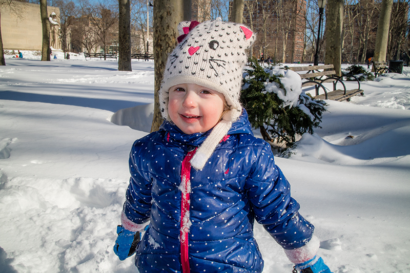
There’s nothing like a fresh snowfall to make a landscape truly dramatic! Snow is an inspiring photographic subject, whether you’re shooting mountain vistas, or single flakes. But it’s also a tricky subject, and many photographers find that the glowingly bright snow scene in front of their lens mysteriously turns into a depressingly gray photo after they take the shot. This article explains why that happens, and how to avoid it, for wonderful snow photos this winter season!

The biggest challenge when photographing snow lies in your camera’s metering system.

No matter how sophisticated the metering in an SLR camera is, it’s engineered to assume it’s reading “normal” subjects, of an “average” brightness. Photograph a landscape in summertime, with green grass, dark green trees, blue sky and white clouds, and the different brightness levels in the scene often average each other out. Much of the time, the meter will get these scenes absolutely correctly exposed. In simplified terms, it does this by averaging bright and dark parts of a scene, so the final exposure renders the overall brightness almost a middle shade of gray.

You may have heard the term “18% gray,” a middle shade of gray which, technically speaking, reflects 18% of the light striking it. This has been a universal reference point in photographic exposure meters for decades.

Just to clarify what that means: Middle gray is roughly the mid-tone on a gray scale — appearing to fall exactly between pure black and pure white. Subjects of this tone reflect about 18% of light (comparatively, white objects reflect nearly 100% and black objects reflect nearly 0%).

Simply put, most cameras assume that everything they photograph reflects 18% of the light, and expose accordingly. Put another way, your camera meters subjects assuming they should be photographically rendered as middle gray.

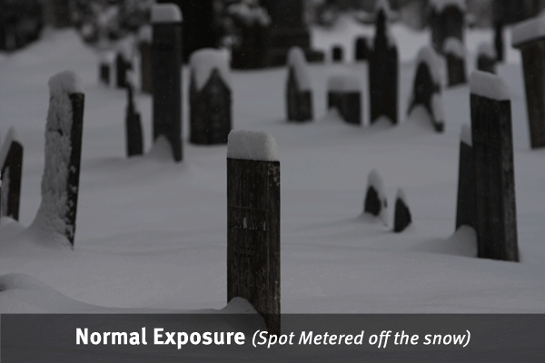
Freshly-fallen clean, white snow is obviously much lighter and more reflective than that, but the camera will automatically try to reproduce it as gray, by underexposing anywhere up to about two stops to correct for what it sees as a too-bright subject. This is exactly why many photographers will find their snow photos to be muddy and underexposed.

In-camera light metering works reasonably well with most subjects, in most lighting situations. However, there are tricky scenes that will baffle most meters — and snow is a classic example.

Most cameras have more than one metering mode (though they all use the basic reflective approach described above). These modes are not always found in every camera, but here are some of the common ones found in the Canon EOS and PowerShot systems:

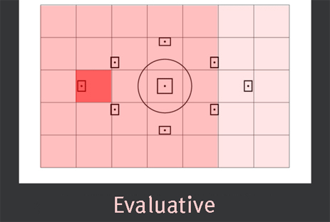
Evaluative: Metering is directly linked to, and concentrated on, the area around the active AF point, whether you’ve focused on something in the center or off-center. Light values measured at the active AF point are compared with light values measured from the metering segments across the remaining areas of the scene, and the camera's metering system attempts to provide an accurate exposure based on that comparison. This metering pattern is often effective when photographing people, but may not be quite as effective when photographing snowy landscapes depending on other elements in the scene. Note that because Evaluative Metering is linked to active AF points, focusing on a different subject may result in a very different exposure — even within the same scene. Note: In the simulated viewfinder, Evaluative mode is shown with the left-most AF point active.

Spot: The most selective metering option, it reads exposure information only from the single exposure zone in the center of the frame (approximately 3% of the total picture area).

Partial: Similar to Spot Metering, but covers a somewhat larger area, reading only the cross-shaped central five metering zones (approximately 10% of the total picture area) — some shooters think of it as a “fat spot.”

Center-weighted Average: This metering mode averages the exposure for the entire metering area, but with greater emphasis on the center metering zones. Unlike Evaluative metering, it does not compare brightness readings from different parts of the scene; it simply reads overall brightness.

Even though Evaluative metering is by far the most commonly-used system by EOS users, when using one of the EOS Creative Zone exposure modes (M, Tv, Av or P), you can select from any of the metering modes offered on your camera. If you prefer to shoot in the Basic Zone exposure modes (Full Auto, Portrait, Landscape, Close-up, Action, etc.), the default mode is usually Evaluative. This is also true in PowerShot cameras — although note that when Face Detection is turned on, any faces in the scene will have exposure priority.

When photographing snow, any of these modes may be used effectively, depending on the overall scene. For example, if there is some contrast between the snow and the rest of the objects in the scene, then Evaluative metering may be ideal because it will emphasize the exposure for whatever you are focusing on — even if it’s off-center.

If the overall scene is evenly lit and of generally even brightness, then Center-weighted Average will work well to give a good overall exposure.

Spot and Partial metering will work well with subjects that have more extreme contrast, and/or when you want to carefully read one part of a subject or scene, and don’t want another part to ‘confuse’ the meter. Either way, they let you meter only a small part of the scene. These metering patterns are very useful when used in combination with the Auto Exposure (AE) Lock button found on most digital SLRs.

Unfortunately, even when the camera ‘accurately’ determines the correct exposure using the metering mode of your preference, with a subject like snow you will often see underexposed results. If and when this happens, however, you have a tool in your camera to deliberately lighten your pictures, and have the white snow properly rendered. That tool is Exposure Compensation.

Exposure Compensation (EC) is the most important — and often, the easiest — way to get around your camera’s tendency to underexpose bright subjects, and overexpose dark ones. It’s also very useful for photographers who are new to Creative Zone shooting (again, the P, Tv, Av, and M settings on your Mode Dial) because it doesn’t require extensive knowledge of f-stops or shutter speeds.

Exposure Compensation lets you deliberately lighten or darken your exposures. You can vary the amount of compensation, anywhere from plus or minus 1/3 of a stop (often, a barely noticeable difference) up to plus/minus three full stops, which will significantly change most images. Using “plus” compensation adds light, so it always deliberately lightens images you’re about to take.

Keep in mind that to use Exposure Compensation (and many other features), your camera has to be in a “Creative Zone” exposure mode… that is, the P, Av, Tv, or M settings on your camera’s Mode Dial. If your camera is set to one of the full-automatic settings, you can’t change exposure, and any Compensation you may have previously dialed-in while in a Creative Zone mode will be ignored.

You can also bracket several shots in a row, with each image of a slightly different exposure using the Auto Exposure Bracket (AEB) function.

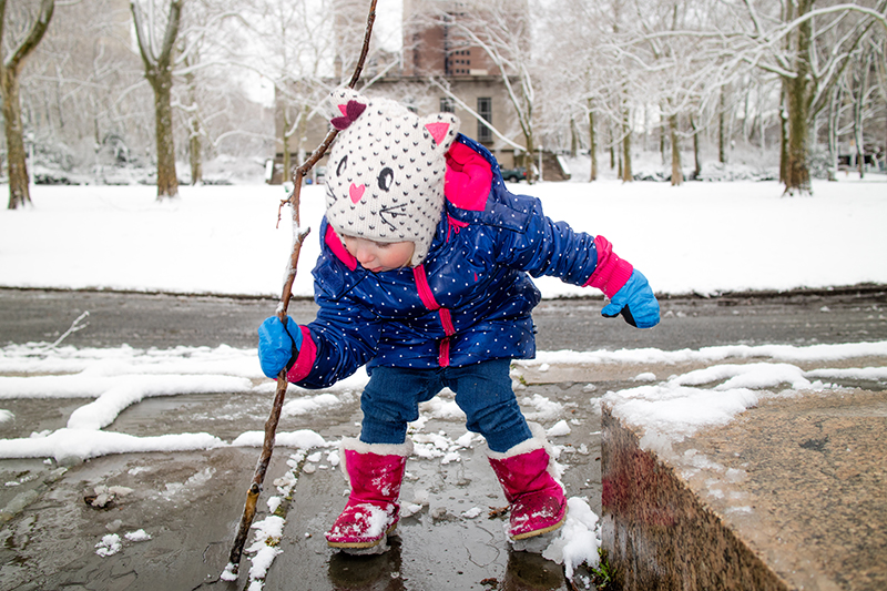
When photographing snow, you’ll want to experiment with adding more exposure, anywhere from +1/3 to +2 stops EC may work, so play around until you find what you like or try using AEB to ensure variety in exposure levels.

Another approach is to shoot RAW images, which provide additional control over exposure compensation on a computer (bonus: you'll be in the warm comfort of your home instead of out in the cold!). However, understand that even when shooting RAW images, it's still necessary to start out with an exposure that's reasonably accurate out-of-camera — and we strongly recommend using Exposure Compensation to lighten snow images whenever it’s needed.

White Balance settings adjust the camera for the overall color character of the light source you are shooting in, so images can have a neutral rendition that properly renders colors in the scene. Many Canon EOS photographers let the camera read light and adjust this automatically, with Auto White Balance (AWB). There are also fixed, pre-set white balance settings, such as Daylight, Cloudy, Shade, and Tungsten.

Many cameras also allow shooters to take a custom White Balance, or even dial in a specific color temperature (measured in degrees Kelvin) to better match your scene, particularly for unusual or mixed-lighting scenes that are not covered by any of the preset options seen here.

Photographing snow implies you will be outside. However, differences in time of day, geographic region, and weather conditions can make a huge difference in the color temperature of your light source — even though the ‘light source’ in this case is always the sun, which means that your White Balance may need to be adjusted, and the preset for 'Daylight' may not always look the best.

The preset White Balance options are pretty accurate, but you have to remember to use the one that most closely matches your light source, and weather conditions. On sunny days with clear blue skies, it’s common to have snow seem to pick up a slight blue tint; experiment with the Cloudy or Shade WB settings to warm-up the overall color and neutralize that blue color cast.

If you shoot RAW images, you can change your White Balance while editing, regardless of your camera settings at the time of shooting. But it still makes sense to deliberately set the proper white balance, or at least one that gets your color close, before you take the picture.

Another reason snow poses a challenge is because any white subject photographed in reasonably bright light is at risk of losing detail with even slight overexposure. Worse yet, once a scene has overexposed highlights, there is often little that can be done in photo editing to bring that detail back. Luckily, our current line of EOS digital SLRs offers a number of functions to help photographers avoid these unfortunate ‘blown out’ highlights.

One easy-to-use, and very effective feature is Highlight Tone Priority (HTP). This innovative image-control feature takes advantage of the expanded tonal range found in newer EOS cameras to achieve up to one stop more detail in bright highlight areas — without effecting the overall exposure or underexposing the rest of the scene.

HTP can only be used in the Creative Zone exposure modes (again, P, Tv, Av, M, or A-DEP on your mode dial), and once it’s turned on, the effect will automatically be applied to JPEG images and even HD video files in-camera. Two notes for RAW image shooters:

• Highlight Tone Priority will be applied (if set in-camera) to RAW images if they are processed in Canon’s Digital Photo Professional software
• HTP is usually ignored if other third-party software is used to process EOS RAW image files, even if HTP was set in-camera

Please note that when HTP is active, the highest and lowest ISO settings of your camera may not be available. Some EOS models have Highlight Tone Priority control in the Shooting Menu; on other models, it’s within the Custom Functions menu.

In addition to Highlight Tone Priority, you can also manage your highlights during playback: by checking image histograms, and using the optional Highlight Alert function.

A histogram is a chart that represents the distribution of pixel brightness in each image. It is visible on the rear LCD screen during Live View shooting, or during playback, and is a very useful way to evaluate exposure. Histograms are sort of mountain-shaped; the height of each peak indicates how many pixels were recorded at particular brightness levels. The most important part, however, is how the display looks side-to-side. The left side of the chart represents shadow tones in the image; the right side represents bright highlight areas, and the center represents mid-tones.

Note that the pixels on the right side of the Histogram are cut off, which indicates overexposure.

Reading a histogram properly helps photographers determine the appropriate exposure for the scene, and whether they are at risk of severe under- or overexposure. When photographing snow, two things to keep in mind as you look at a histogram when playing-back an image:

1. If the scene is mostly snow, but the histogram shows a big “mountain” in the middle area of the histogram, it usually means the camera has tried to make the snow middle-gray. This is your warning to set Exposure Compensation in the “plus” direction, and take another picture… your goal is snow that appears white, not gray!
2. If snow has been properly-exposed and rendered a white tone in your image, you’ll probably see a lot of information to the far right side of the histogram. As long as it’s not being cut-off by the right side of the graph, this is a good sign… the histogram info is telling you your white subject is being reproduced as a white tone in your digital image.

But, if your histogram shows portions of the graph that appear to get cut off on the far right, that means portions of your scene are severely overexposing to the point that detail may be washed out. This is a warning that your exposure should be adjusted. If you see this, try applying minus Exposure Compensation, until you see that no part of your histogram is cut off at the right edge.

Another way to check for overexposure during LCD monitor playback is with a feature called Highlight Alert. When active, this alert causes all portions of the frame on the verge of overexposing to blink on and off. This is an optional feature that can be enabled or disabled on the Playback menu of most of our EOS digital models; with EOS Digital Rebel models, it’s displayed whenever the histogram is on-screen during Playback.

If you plan to shoot outdoors in the cold for an extended period of time, please consider the following precautions to ensure the safety and functionality of your camera equipment:

• Cold batteries die faster, especially in temperatures below the freezing point, so keep your batteries warm. Keep the camera relatively warm, and when possible, resist the temptation to leave it or your camera bag in cold places like the trunk of a car or unheated areas of a building for long periods of time. Also, bring spare batteries, fully-charged, and keep those warm in your pockets until ready for use
• Give your camera equipment time to acclimate when going from cold to warm temperatures. Otherwise, you risk condensation build-up, which can damage lenses as well as internal digital camera components. Gradually introduce it to warmer temperatures. One example would be to gently warm equipment using a car’s heater — not too much, however! — after cold-weather shooting, prior to bringing the gear into a heated building.
• Another trick to prevent condensation build-up when moving from cold to warm temperatures is to seal your camera in an airtight plastic bag (such as a Ziplock). Seal the camera completely inside of the bag BEFORE moving indoors, and condensation should form on the bag rather than the camera. Leave the camera inside the bag until it's had a chance to fully warm up to room temperature.
• If you anticipate mild snow or rain while shooting, waterproof your camera with plastic bags. Bring lens cloths or lint-free tissues to wipe off any moisture that might build up on the lens from melting snowflakes.
• Keep your hands warm. Invest in fingerless gloves with a fold-back mitten top, so you can access camera controls while keeping your hands as warm as possible in between shots.

- Ordered List Item

======Animating Falling Snow====== * Unordered List Item

Author: ctown4life

Tools Needed

• Any image editing program (such as Photoshop)

Support Files

Introduction

Step 1 - Create Planes

Step 2 - Parenting the Planes

Step 3 - Painting the Opacity Maps

Step 4 - OpenGL

Step 5 - Create snowCam

Step 6 - Create D-Former

Step 7 - The Timeline

Step 8 - Animate the Snow Planes

Step 9 - Animate D-Former part1

Step 10 - Animate D-Former part2

Step 11 - Customizing and Final Notes